Project 10 · Numerical analysis and computing

The race between solvers

Make a simulation twice as sharp and it can take many times longer. Race the methods and find out which wins, and when.

Instructions (PDF)Starter code (10_solver_race.py)

Math: Algebra II, logarithms; some programming helps
You need: A laptop; some programming helps
Tools: Python; a mentor's Apple Silicon or NVIDIA machine for the GPU stage
Solver: Poisson, 2D; sbp-sat-suite for multigrid and GPU

The question

Doubling a simulation's resolution makes a basic solver far slower. How do accuracy, iteration count and run time scale, and at what size do higher-order methods, multigrid and GPUs actually pay off?

Objectives

Twelve weeks, in the four stages every TopEdu project follows. Your mentor reviews each checkpoint before you move on.

Weeks 1 to 3
Learn to trust the model
Run 10_solver_race.py until its CHECK line says PASS, and explain every line of it to your mentor. Then reproduce a known answer: The solution has a known exact form, so you can measure the real error. Our test run gives rates of 2.00, 3.00 and 4.95 for orders 2, 4 and 6. Part of your project is explaining why the labelled order and the measured rate differ.
Checkpoint: you reproduce a known answer and report how close you got.
Weeks 4 and 5
Ask your own question
Narrow the question above to one sentence that could turn out to be wrong, and write your prediction before you run anything. The first experiments below are a place to start.
Checkpoint: a one-page plan with your question and prediction.
Weeks 6 to 9
Run it, then measure the world
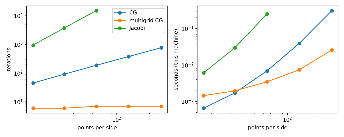
Measure error and iterations as the grid grows for orders 2, 4 and 6, then race conjugate gradients against multigrid, and CPU against GPU, with the sbp-sat-suite tools. Then step away from the screen: time everything on real hardware and fit the power laws yourself. In our test, CG needed 127 to 416 iterations from 65 to 513 points while multigrid stayed near 15, and multigrid won on time only past about 257 points. Your machine's break-even point is your own result.
Checkpoint: one chart comparing your model with reality.
Weeks 10 to 12
Explain the gap, and share it
Work out why your model and your measurements disagree, test at least one explanation, and write it up yourself. Say which numbers came from the starter and which from the lab. Keep the honest limit in view: the online lab covers conjugate gradients only. Multigrid and GPU runs use the sbp-sat-suite tools with a mentor.
Checkpoint: a final paper, your code and a ten-minute talk.

The data

What the lab lets you change, how the project was checked before we listed it, and what the starter prints on a laptop.

Settings in the online lab

Setting	Range	Starts at
Grid points per side	9 to 129	33
Accuracy order	2 to 6	4

Checked on the research solver

Solver (Poisson, 2D; sbp-sat-suite for multigrid and GPU)	order 2: rate 2.00, iterations 29 > 52 > 91 > 154; order 4: rate 3.00, iterations 31 > 61 > 113 > 200; order 6: rate 4.95, iterations 36 > 77 > 145 > 265
Known answer	error falls at least as fast as the order's boundary rate (order 2 gives about 2)
Error	0.03% (limit 10.00%): passed

What the starter prints

From the run that built this page. Timings depend on your computer; the CHECK line must say PASS.

points   method          iterations   seconds   max error
    17   CG                     45     0.001   3.62e-04
    17   multigrid CG            6     0.001   3.62e-04
    17   Jacobi                950     0.006   3.62e-04
    33   CG                     92     0.002   9.07e-05
    33   multigrid CG            6     0.002   9.07e-05
    33   Jacobi               3750     0.030   9.07e-05
    65   CG                    187     0.007   2.27e-05
    65   multigrid CG            7     0.003   2.27e-05
    65   Jacobi              15050     0.250   2.27e-05
   129   CG                    379     0.039   5.68e-06
   129   multigrid CG            7     0.007   5.68e-06
   257   CG                    768     0.310   1.42e-06
   257   multigrid CG            7     0.026   1.42e-06
measured convergence rate: 2.00 (second-order differences should give 2)
CHECK convergence rate near 2 -> PASS (limit 2 +/- 0.1)

Iterations and seconds for each solver as the grid grows

The starter code

One Python file that needs only numpy and matplotlib. Run python3 10_solver_race.py --show to see the plots. How to set up.

The model

The test problem: -laplacian(u) = f on the unit square, u = 0 on the edge, with f chosen so the exact answer is u = g(x) g(y), g(s) = s (1 - s) e^s. Knowing the answer lets you measure the real error of every method. (The lab uses u = sin(pi x) sin(pi y). Try it here, in problem(): CG then finishes in one iteration. Why?)

This file races three ways of solving the same grid equations (plain second-order finite differences): Jacobi: each point becomes the average the equation wants. Simple, and very slow on big grids. Conjugate gradients: the standard method for this kind of system; its iterations grow with the grid. Multigrid (V-cycle): fixes smooth errors on coarser grids; its iterations should stay flat.

What it does

Stage 1: run it. It checks that the error falls like h^2 (rate near 2). The CHECK line should say PASS.
Stage 2: time everything as the grid grows, fit the power laws, and find your own machine's break-even point. The online lab uses higher-order SBP-SAT methods; sbp-sat-suite has a mentor-run multigrid and GPU version.

Your first experiments

From the YOUR TURN list at the bottom of the file. Write your prediction in your log before you run each one.

Predict first: if CG's iterations grow like n^p, what is p? Fit it from the table (polyfit on the logs). Do the same for time. Why does time grow faster than iterations?
Add 513 points. From what size does multigrid win on time here? Compiled code (sbp-sat-suite) shifts that point, because each method's cost per iteration changes. Your machine's break-even point is your own result.
In the online lab, run orders 2, 4 and 6 at 17, 33, 65 and 129 points and measure each order's rate. Order 4 measures about 3 in our tests. Why might the boundary be the reason?
With a mentor: race CPU against GPU in sbp-sat-suite. Report where your numbers differ from its README.

Download 10_solver_race.py All ten (.zip)Instructions (PDF)

The real world

Time everything on real hardware and fit the power laws yourself. In our test, CG needed 127 to 416 iterations from 65 to 513 points while multigrid stayed near 15, and multigrid won on time only past about 257 points. Your machine's break-even point is your own result.

The honest limit

The online lab covers conjugate gradients only. Multigrid and GPU runs use the sbp-sat-suite tools with a mentor.

Want to work on this one?

Members run it on the research solver in the lab and choose a mentor to guide them.

Open in the lab Apply for membership